For more information or if you need help retrieving your data, please contact Weights & Biases Customer Support at support@wandb.com
A practitioner’s guide to machine learning pipeline architecture, MLOps maturity and the tooling that closes the gap between experiment and production.
A recommendation model goes live after months of development. Validation metrics are strong, the demo impressed stakeholders, and the team ships it with confidence. Six weeks later, a product manager notices engagement has dropped and files a ticket. The data science team investigates. The model is still running, but the data feeding it had quietly shifted weeks earlier. No alert fired. No dashboard changed color. The only reason anyone noticed was a product manager who happened to look at the numbers.
That scenario plays out across industries more often than most teams admit. The model was not the problem. The system around the model was. There was no monitoring to detect drift, no versioning to confirm what was actually deployed, and no record of when the model was last validated. Answering basic questions ttakes days of digging through notebooks and chat threads.
A mature MLOps pipeline is what prevents this.
In business terms, an MLOps pipeline is the operating system that connects raw data, model development, review controls, and deployment decisions into a governed, repeatable path from idea to production value. For directors and managers, that matters because the real cost of ML is rarely the training run. The cost shows up in delays, rework, unclear ownership, audit friction, and models that degrade without visibility.
When teams standardize their pipeline, three things improve together:
This is the domain of MLOps (machine learning operations): the discipline of making ML work more like a governed engineering system. Tools like Weights & Biases give teams one place to track experiments, datasets, model artifacts, and production behavior across the pipeline, turning governance from a procedural requirement into a property of the workflow itself.
An MLOps pipeline is a defined, reproducible sequence of steps that takes data through preparation, training, validation, deployment, and monitoring in a way that can be automated, versioned, and audited. It is designed for production, not for exploration.
That sounds straightforward until you look at how most ML work actually starts. A team explores data in notebooks, writes utility scripts, trains model variants, exports a checkpoint, and hands it to another team with a mix of screenshots, assumptions, and tribal knowledge. The result can work once. It breaks the moment someone else needs to reproduce it, or an auditor asks where the training data came from.
A pipeline is what happens when you stop treating the notebook as the deliverable and start treating it as a sketch for the real thing.
The scale of what surrounds the model is easy to underestimate. In their 2015 NeurIPS paper, “Hidden Technical Debt in Machine Learning Systems,” Sculley et al. found that the core ML code in a mature production system accounted for roughly 5% of the total codebase. The remaining 95% is data ingestion, feature pipelines, serving infrastructure, configuration management, monitoring, and what the authors call glue code: the brittle connective tissue that holds everything together.
That finding has a corollary, the CACE principle: “Changing Anything Changes Everything.” In standard software, changing a function affects the functions that call it. In an ML system, changing an input signal, a sampling strategy, or a feature definition can silently alter model behavior across slices of the distribution in ways that are difficult to predict. An MLOps pipeline with proper versioning and experiment tracking is the structural defense against that kind of change propagating undetected to production. The full paper is available from the NeurIPS proceedings.
Data is cleaned each sprint manually. Retraining local. Evaluation by eye. Deployment via a shared script that only one person understands. Works once. Cannot be reproduced or audited.
Data ingestion triggered on schedule. Features versioned. Every training run automatically logs metrics and artifact references. Validation gates run before promotion. Any engineer can trace a production model back to the exact training run and dataset version.
The major cloud providers converge on the same definition: a repeatable flow composed of defined steps, dependencies, inputs, and outputs rather than a one-off script. Azure Machine Learning, Amazon SageMaker Pipelines, and Google Vertex AI Pipelines each offer managed orchestration with this foundation.
A data pipeline moves and transforms data from source systems into a warehouse or lake, cleaning and structuring it so analysts can query it. It cares about completeness, freshness, and schema correctness. That is the right scope for a data pipeline.
An MLOps pipeline sits atop a data pipeline and extends beyond it. It trains models on that clean data, evaluates their statistical behavior, versions the artifacts produced, deploys them into the serving infrastructure, and monitors their behavior as the world changes. It introduces concepts that a data pipeline has no mechanism to handle: model versioning, hyperparameter tracking, bias evaluation, drift detection, and model approval workflows.
The most damaging failure mode at this boundary is training-serving skew. This occurs when the feature computation logic at training time produces different values than the same logic at inference time. Training typically runs as a batch Python job against historical data. Inference runs as a real-time microservice, often in a different language or framework. Differences as small as timezone handling, null value imputation, or floating-point rounding can shift feature distributions enough to cause significant loss of accuracy. Google’s own Rules of ML documentation cites training-serving skew as a source of dramatic performance setbacks: fixing a single feature discrepancy in Google Play improved app install rates by 2% at scale.
A mature MLOps pipeline either enforces shared feature computation code across training and serving or routes both environments through a feature store that guarantees numerically identical outputs. A data pipeline has no reason to care about this distinction. An ML pipeline must enforce it.
| Dimension | Data Pipeline | MLOps Pipeline |
|---|---|---|
| Primary output | Clean, queryable data | Trained, versioned, deployed models |
| Versioning concern | Schema and table versions | Dataset, feature, model, and run versions |
| Failure modes | Missing data, broken transforms | Above + drift, bias, and accuracy degradation |
| Governance needs | Lineage, access control | Above + model approvals, audit trails, explainability |
| Typical owners | Data engineers | ML engineers, MLOps engineers, data scientists |
| Continuous training? | No | Yes: models retrain as data and concepts evolve |
| Training-serving skew? | Not applicable | A primary failure mode requiring explicit prevention |
For leaders making staffing and tooling decisions, owning a mature data platform provides a strong foundation, but it does not deliver an ML pipeline. The survey by Paleyes, Urma, and Lawrence, published in ACM Computing Surveys (2022), found that data management issues and deployment-stage problems are the most frequently cited challenges in real-world ML deployment case studies. Both categories require ML-specific controls that data engineering alone cannot provide.
MLOps applies CI/CD principles to machine learning: automation, testing, versioning, and monitoring applied to the full model lifecycle. The operational case for it is simple. Vela et al. (2022), publishing in Nature Scientific Reports, ran 20,000 experiments across 32 datasets in healthcare, weather, traffic, and finance. They found temporal accuracy degradation in 91% of model-dataset combinations. Models left unchanged decay. The only variable is how fast and whether anyone detects it.
Google’s MLOps: Continuous Delivery and Automation Pipelines in Machine Learning reference architecture defines three maturity levels that give teams an honest assessment framework:
Notebooks, manual retraining, no CI/CD for ML. Data science disconnected from ops. Most organizations start here and believe they are at Level 1.
The ML pipeline is automated end-to-end. Continuous training on new data. Feature store and metadata tracking in place. Model validation gates before deployment.
Full CI/CD for pipeline components. Automated tests for data, models, and infrastructure. Multiple teams deploy models independently on a repeatable release path.
The most reliable indicator of Level 0 MLOps is this: retraining requires a human to decide and manually trigger it. If that describes your current state, be honest about it. Level 0 is a starting point, not a failure. But treating it as Level 1 means the investment decisions to close the gap never get made.
A concrete assessment tool is the ML Test Score rubric published by Breck et al. (2017) at Google. It defines 28 specific tests across four categories: data and feature tests, model development tests, ML infrastructure tests, and production monitoring tests. Running through this rubric takes a morning and produces an honest gap analysis of your current pipeline against a production-ready standard. Most teams discover they are strong in model development tests but weak in data, infrastructure, and monitoring tests.
Vela et al.'s finding that 91% of model-dataset combinations degrade over time does not mean 91% of deployed models are failing right now. It means the default outcome, without monitoring and continuous training, is degradation. The pipeline is what changes the default.
The stages of an MLOps pipeline follow the natural lifecycle of a model. What makes a mature pipeline different from an ad-hoc process is not the stages themselves but that each one is defined, automated, and observable.

![]()
Every model failure, traced back far enough, leads to a data problem that the MLOps pipeline failed to catch. Wrong schema accepted silently. A source that changed its timestamp format three months ago. Training data filtered differently from what production would see.
The first stage of an ML pipeline ingests and curates data from operational systems, event streams, and data warehouses into versioned, auditable datasets. This is where the pipeline picks up from where the data pipeline leaves off.
One failure mode that passes all standard data quality checks is temporal leakage. In time-sensitive prediction tasks (churn, fraud, demand), a feature computed over a 30-day lookback window might accidentally include data from after the prediction date if the pipeline’s timestamp logic has a bug. The model trains on features it would not have at inference time, achieves strong offline metrics, and fails in production.
Point-in-time correctness means every feature is computed using only the data that existed at the prediction timestamp. Feature stores enforce this by design. Building it into ad-hoc pipelines retroactively is significantly harder, which is why data ingestion is worth engineering properly the first time.
W&B Artifacts tracks dataset versions with full metadata: source, schema, row count, timestamp, and the job that produced it. Every subsequent training run links to the exact dataset version it consumed, making temporal leakage auditable after the fact. See the W&B experiment tracking documentation for how artifact lineage works in practice.
![]()
Feature engineering transforms raw fields into the inputs a model can use. It is also where the training-serving skew problem originates and needs to be solved.
A production feature pipeline must serve two fundamentally different interfaces. The offline interface handles training: it operates in batch, accesses months of historical data, and must be point-in-time correct. The online interface handles inference: it operates on a single record, must return in milliseconds, and serves from a low-latency store. Teams that build one interface without the other hit predictable problems: a batch-only pipeline cannot support real-time serving; an online-only pipeline cannot generate point-in-time correct training sets. The two interfaces require different infrastructure but must produce numerically identical values for any given input. Any divergence is training-serving skew.
Feature importance drift is an underused early warning signal. If the features the model weights most heavily start shifting in distribution before the model’s aggregate accuracy visibly drops, you get a leading indicator of coming degradation rather than a lagging one. Tracking feature importance across training runs and comparing feature distributions at training time against those at inference time gives teams a head start.
W&B Artifacts versions computed feature sets alongside their lineage, linking each feature dataset to the pipeline run that produced it and the raw data it consumed. W&B Tables enables distribution visualization, making it practical to compare feature distributions across dataset versions before training begins.
![]()
Training is the stage most people visualize when they think of ML work: experiments, hyperparameter tuning, loss curves. What organizations consistently underestimate is the infrastructure required to make training reproducible and comparable at scale.
The CACE principle from Sculley et al. (2015) — Changing Anything Changes Everything — explains why experiment isolation matters more in ML than in standard software. In an ML system, changing an input signal, a feature’s computation, a sampling strategy, or a data preprocessing step can change model behavior across distribution slices in ways that are hard to detect and harder to attribute. Two experiments are only meaningfully comparable if all unintentional variables are held constant. Without systematic tracking, you are often not measuring the effect of your intended change.
Sculley et al. also identified undeclared consumers as a specific ML debt pattern: other systems that depend on a model’s outputs without the producing team’s knowledge. As models are used more broadly, their outputs become implicit inputs to other pipelines. A change that improves the primary model may silently break a downstream consumer. Dependency documentation and versioned model APIs are the structural solution.
Run configs noted in comments. Metrics in a shared spreadsheet that is six versions behind. Final model selected by memory. Impossible to reproduce. No audit trail connecting production model to training run.
Every run logs hyperparameters, dataset version, environment, system stats, and metrics automatically. Promotion references a specific run ID. Any team member can reconstruct any experiment from the artifact graph.
W&B Experiments logs every run automatically: metrics, loss curves, hyperparameters, system stats, and artifact references. W&B Sweeps automates hyperparameter search, running multiple configurations in parallel. Both tools enforce the isolation required by the CACE principle. Full documentation at docs.wandb.ai/guides/track.
![]()
Statistical accuracy on a held-out test set is necessary for promoting a model to production. It is not sufficient.
Goodhart’s Law states that when a measure becomes a target, it ceases to be a good measure. In ML, this manifests as models that optimize for the logged metric in ways that do not translate to business value: a recommender system that maximizes click-through rate by surfacing clickbait, or a fraud model that achieves 99.9% accuracy by predicting ‘not fraud’ for everything in a class-imbalanced dataset. The practical defense is a multi-metric evaluation with pre-committed thresholds, set before training begins rather than tuned to match whichever model was just trained.
The ML Test Score rubric from Breck et al. (2017) formalizes this. It’s 28 tests across four categories, including checks that the model performs consistently on important data slices, that it outperforms a simple baseline, that training is deterministic for debugging, and that the evaluation infrastructure itself is tested. These tests belong in automated validation gates, not in monthly review meetings.
Shadow mode deployment is an underused pre-production validation technique. The candidate model runs in the production environment, but its outputs are logged and not served to users. Production traffic is duplicated: the live model serves responses while the shadow model processes an identical copy and records its predictions. This gives the candidate model its first exposure to real data distributions, real latency constraints, and real edge cases before it affects anyone.
W&B Reports creates shareable, version-locked evaluation summaries (performance metrics, bias analysis, baseline comparisons) that serve as approval artifacts. W&B Models formalizes promotion: a model moves from 'staging' to 'production' through a defined review workflow with a full record of who approved it, when, and based on what evidence. See the W&B model registry documentation for how staged promotion works.
![]()
Deployment is where ML engineering and software engineering collide, and where organizational friction peaks. Application teams own the services. ML teams own the models. The handoff (‘here is a model artifact, please integrate it’) is often the weakest link, especially when there is no standard for how models are packaged or versioned.
AWS documents a combined shadow-and-canary pattern in their end-to-end MLOps pipeline reference: the shadow model processes a copy of live traffic while the canary model serves a small percentage of users. The combination gives two independent signals before full rollout: production data behavior (shadow) and real user impact (canary).
Canary analysis for ML differs from standard software canary releases in one important way: the success criterion is not just service health (latency, error rate) but model quality metrics (prediction distribution, confidence calibration, outcome agreement with the champion model). Statistical significance testing on prediction distributions distinguishes real behavioral differences from noise before traffic increases.
![]()
Most organizations treat monitoring as optional, only to regret it later. Vela et al. found temporal degradation in 91% of model-dataset combinations tested. Models degrade by default. Monitoring is what changes the default outcome.
Treating all three identically works for covariate drift but misses concept drift until the damage is significant. Diagnosing which type is occurring before choosing a response is a material operational improvement.
The Population Stability Index (PSI) is one of the most widely used drift metrics. It measures the divergence between the training distribution and the current serving distribution for a given feature. Industry-standard thresholds: PSI below 0.1 is stable; 0.1 to 0.2 warrants investigation; above 0.2 indicates significant drift and should trigger retraining. These are rules of thumb, not statistically derived absolutes — feature importance moderates how aggressively a given PSI value should be treated.
The right-censoring problem in feedback loops is less discussed but equally important. When a model’s decisions determine which outcomes are observed — a loan model that only sees repayment behavior for approved applicants, a content moderation model that only has labels for flagged content — the feedback loop is structurally biased. Retraining on observed outcomes alone encodes the model’s own past decisions into its future behavior. Solutions include counterfactual logging, inverse propensity weighting, and randomized exploration (occasionally approving near-miss cases to observe outcomes that would otherwise be invisible).
SLA tracking, incident response playbooks, and compliance reporting all require production monitoring data. In regulated environments, demonstrating that a model's performance was actively monitored and that degradation triggered a defined response is often a compliance requirement. An observability gap at this stage is a regulatory gap.
The building blocks of a modern machine learning pipeline architecture are consistent across cloud providers, even if the product names differ. The gap in most organizations is not missing components — it is missing integration and missing metadata.

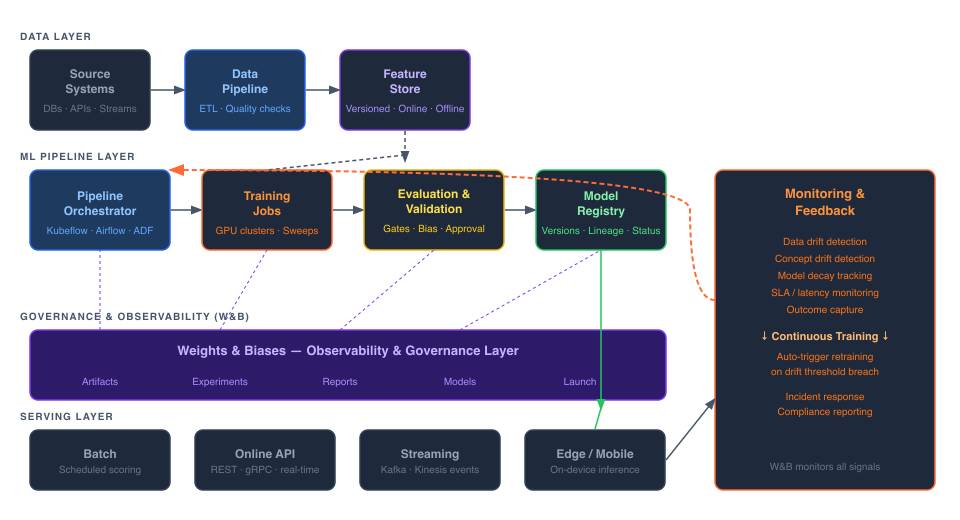
| Layer | What It Contains and Why It Matters |
|---|---|
| Data Layer | Source systems, ETL pipelines, and feature store. The feature store’s offline API provides point-in-time correct training data; its online API serves the same feature logic at inference time. This dual-API design is the architectural solution to training-serving skew. |
| Orchestration Layer | Workflow engine (Airflow, Kubeflow, Azure Data Factory, SageMaker Pipelines) that runs pipeline steps in order, handles retries, and manages dependencies between stages. |
| Experiment and artifact layer | Runs, parameters, datasets, model versions, and lineage. This is the metadata graph: a first-class architectural component that links every production model to its training run, dataset version, and feature definitions. |
| Release layer | Validation rules, approval gates, model registry, packaging, and deployment automation. The registry is the control point that turns ML delivery into a managed process. |
| Observability layer | Drift monitoring, prediction distribution tracking, latency and throughput metrics, audit trails, and retraining triggers. W&B operates across both the layer and the experiment/artifact layers as a unified governance surface. |
Google Vertex AI, Amazon SageMaker Pipelines, and Azure Machine Learning pipelines each implement these layers with different managed services but share the same architectural logic. The key insight is that the lineage graph — the metadata connecting every artifact to the run that produced it — is not a reporting feature. It is the operational foundation of reproducibility, debugging, and compliance.
The 5% ML code finding from Sculley et al. is widely cited, but its implication is less often acted on: if the model is 5% of the system, optimizing only the model while leaving the 95% unmanaged is a category error. The research paper identified specific technical debt patterns that explain where much of that 95% goes.

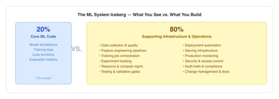
These patterns do not emerge from bad engineering. They emerge from the normal pace of ML experimentation applied to systems that were never designed for production scale. The full catalog is in the Sculley et al. (2015) paper. MLOps platforms and shared pipeline infrastructure reduce accumulation by making the hidden visible: tracked artifacts, versioned components, and automated validation make each of these debt patterns detectable before they compound.
When estimating ML project timelines and headcount, explicitly account for the 95%. If your plan covers model development, you have budgeted for 5% of the work. The missing 95% will appear as overtime, delays, and post-launch incidents.
Consider a predictive maintenance system for industrial equipment. Sensors on manufacturing machines stream temperature, vibration, and pressure readings. The goal is a model that predicts equipment failures 24 to 72 hours ahead, giving maintenance crews time to intervene before unplanned downtime.
AWS documents a structurally similar pipeline for visual quality inspection at the edge (part 1). The predictive maintenance example shares the same architectural logic and illustrates how all six stages interact in a real production context.
Most pipeline pain does not come from a single missing feature. It comes from context split across too many tools: training logs in one place, dataset versions in a spreadsheet, model comparisons in ad-hoc notebooks, deployment records in chat threads, and audit trails reconstructed manually. The cost is not obvious until a compliance review, an incident, or a new team member asks a simple question that takes two days to answer.
Pipeline Stage | Gap Without It | W&B Capability |
Data ingestion | No dataset versioning; temporal leakage is invisible until production failure | Artifacts: versioned datasets with schema, lineage, and run provenance |
Feature engineering | Feature logic changes silently; training-serving skew undetected | Artifacts + Tables: feature version lineage, distribution profiling, run-to-run comparison |
Training | Runs not logged; CACE violations undetectable; not reproducible | Experiments + Sweeps: automatic logging, hyperparameter search, full dependency graph |
Evaluation | Promotion decisions are undocumented; Goodhart’s Law effects are unchecked | Reports + Models: version-locked evaluation summaries, formal staged promotion workflow |
Deployment | No reproducible deploy; rollback requires manual reconstruction | Launch + Artifacts: standardized deployments, versioned model packages, one-click rollback |
Monitoring | Drift invisible; right-censoring bias accumulates; no compliance trail | Monitoring: distribution comparison, PSI tracking, drift alerts, governance dashboards |
W&B is a horizontal layer, not a replacement for the underlying infrastructure. It works alongside Azure ML, SageMaker, and Vertex AI, capturing the metadata those platforms produce and making it traceable across the pipeline lifecycle. Full documentation: experiment tracking at docs.wandb.ai/guides/track, model registry at , and model management concepts at docs.wandb.ai/guides/core/registry/model_registry.
The most counterproductive approach to ML maturity is attempting to build the Level 2 architecture all at once. It produces a platform project that delivers nothing to the business for 12 months, generates organizational friction, and is often canceled before the difficult parts are completed.
The more effective approach is to pick one high-value ML use case and build the pipeline properly, including versioned data, tracked experiments, validation gates, and monitoring. Then use that as the template.
MTTD and MTTR are the right operational metrics for ML teams, analogous to what DORA metrics are for software delivery. Most teams measure neither. Teams that do measure them find that the first improvement is almost always instrumentation: you cannot reduce what you cannot detect.
The single highest-leverage first step is adding experiment tracking to your training jobs. It costs almost nothing in engineering time, produces immediate value in reproducibility and comparability, creates the artifact lineage that every more advanced MLOps capability builds on, and gives you the metadata foundation the ML Test Score rubric requires.
The research is consistent. Sculley et al. showed that only 5% of an ML system is model code and identified the specific debt patterns that accumulate in the other 95%. Vela et al. showed that 91% of models degrade over time without active management. Paleyes et al. cataloged the deployment challenges that prevent ML from reaching production in the first place. The common thread is that the model is not the hard part. The pipeline is.
A well-designed machine learning pipeline transforms ML from fragile experimentation into a governed, repeatable capability. It shortens time-to-value by eliminating rework and handoff friction. It improves observability by making evidence available across training, release, and production. It strengthens governance by embedding approvals, lineage, and monitoring into the workflow rather than bolting them on afterward.
The organizations that get this right are not necessarily the ones with the largest ML teams or the most sophisticated models. They are the ones that invested in their pipeline infrastructure: versioned everything, tracked every experiment, formalized every approval, and monitored every production model. Those investments compound. Each new use case is faster to ship and safer to operate than the last.
Pick one production ML pipeline in your organization. Run the ML Test Score rubric against it. Find the single missing layer (experiment tracking, monitoring, model registry, or something else) and fix it end-to-end. That is a more valuable 90 days than designing the perfect MLOps architecture from scratch.